How To Do Data Formatting & Data Handling in Excel?

This practical guide will take you through all the steps involved in data formatting and handling in Excel. Excel’s data handling and formatting features are widely used across industries, including:

• Financial analysts
• Accountants
• Data analysts
• Researchers
• Project managers

All these professionals rely on Excel for tasks like analyzing financial data, tracking expenses, managing budgets, organizing research data, and creating reports. Its versatility makes it a valuable tool for a range of professionals in various roles.

In this manual, we will discuss:

• Autofill and Series
• Introduction to cell references (relative vs. absolute)
• Text to Columns
• Remove Duplicates
• Data Validation
• Find and Replace

Autofill and Series

Autofill in Excel is like a super handy magic trick. Imagine you have a list of numbers or dates that you want to repeat or continue in a pattern. Instead of typing each one out, you can use Autofill to do it for you.

Just enter the first few numbers or dates in a row or column, then click and drag the little square at the bottom-right corner of that cell. Excel will automatically fill in the rest for you, following the pattern it detects. It’s a great time-saver and makes working with repetitive data a breeze!

For example, if you type “1” in cell A1 and then drag the fill handle down, Excel will automatically fill cells A2, A3, and so on with the numbers 2, 3, and so on.

Series is a more advanced version of Autofill that allows you to create more complex patterns. For example, you can use Series to create a list of even numbers, a list of squares, or a list of Fibonacci numbers.

To use Autofill or Series, you first need to select the cells that you want to fill. Then, you can drag the fill handle or use the Series dialog box.

Here is an example for you to understand:

Take an example in which we will try to automatically fill the data in cells horizontally by recognizing the data pattern.

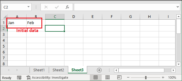
Step 1: We have initially taken the month names as an abbreviation in A1 and B1 cells.

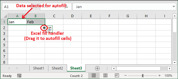
Step 2: Now, select both the cell and hover the mouse at the bottom right corner of the selected cell. A small bold + sign will appear. (This is called Excel Fill Handler.)

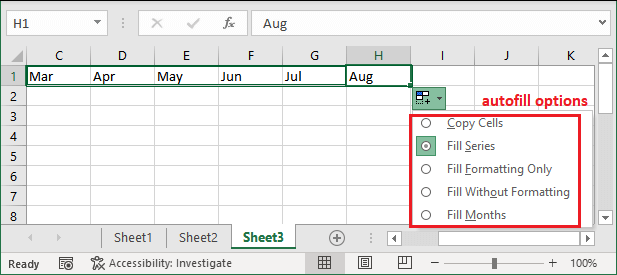
Step 3: Drag the + sign down in the Excel sheet. It will recognize the pattern as month and automatically fill the remaining month name in other cells.

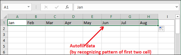
See that the data is generated and placed in cells horizontally. Here, it has inserted a sequence by recognizing the pattern of the first cell and second cell.

Step 4: At the end of the generated values, an Autofill Options box will display.

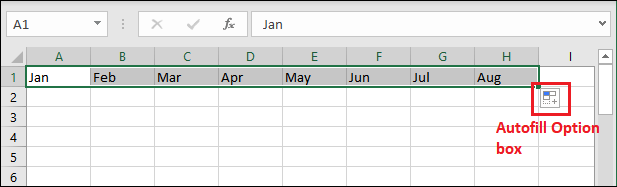
Step 5: Click this Autofill Options box that will show many autofill options.

An Easy Guide to Cell References in Excel: Relative vs. Absolute

When you use formulas in Excel, you often need to refer to other cells to calculate values. These cell references are like instructions that tell Excel where to look for the data you want to use.

There are two main types of cell references: relative and absolute.

1. Relative Cell References:

• A relative cell reference changes when you copy the formula to a new location.
• For example, if your formula is =A1+B1 and you copy it to cell C1, it will change to =A2+B2. This happens because Excel automatically adjusts the references based on the new location.

2. Absolute Cell References:

• An absolute cell reference does not change when you copy the formula.
• You can make a reference absolute by adding dollar signs ($) before the column letter and row number. For example, =$A$1.
• When you copy this formula to a new location, the reference remains fixed. So, if you copy it to cell C1, it will still be =$A$1.
  

Splitting Text into Columns Using Excel’s Text to Columns Feature

Excel’s Text to Columns feature is a powerful tool for splitting text data into separate columns.

For example, if you have a column containing full names like “John Doe,” you can use Text to Columns to split this into two columns, one for first names and another for last names.

Here’s a simple guide to using Text to Columns:

1. Start by selecting the column containing the text you want to split.
2. Go to the Data tab on the Excel ribbon and click on the “Text to Columns” button.
3. In the Text to Columns Wizard, choose how you want to split your data. Common options include tab, semicolon, comma, or space. For names, you’d typically choose space.
4. The wizard will show you a preview of how your data will be split based on your delimiter choice. If it looks good, click “Next.”
5. If your data includes any special formats (like dates or numbers), you can specify how you want them formatted. Otherwise, you can leave this as “General.”
6. Select where you want the split data to appear – either in the existing cells (replacing the original data) or in a new column. Click “Finish” to apply the changes.

Find and Remove Duplicates

Duplicate data is sometimes useful, but it often just makes the data harder to understand.  Finding, highlighting, and reviewing the duplicates before removal is better than removing all the duplicates straightway. 

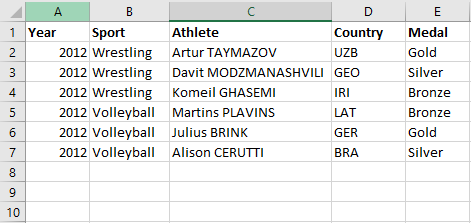
1. Select the range of cells containing duplicate values that should be removed. The best way to remove duplicates is to remove any outlines or subtotals from your data.
2. By selecting Data > Remove Duplicates and then checking or unchecking the columns you wish to purge, you can remove duplicate records.
3. Then click OK.

How to Remove Duplicate Values in Excel

Excel has a built-in tool that helps delete repeated entries in your dataset. Let’s have a look at the steps to be followed to remove duplicates in Excel.

• Step 1: First, click on any cell or a specific range in the dataset from which you want to remove duplicates. If you click on a single cell, Excel automatically determines the range for you in the next step.

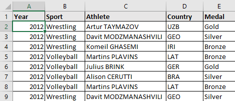
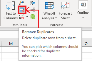
• Step 2: Next, locate the ‘Remove Duplicates’ option and select it. DATA tab → Data Tools section → Remove Duplicates

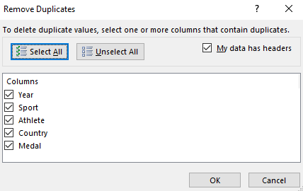
• Step 3: A dialog box appears, as shown below. You can select the columns you want to compare and check for duplicate data. 

In case your data consists of column headers, select the ‘My data has headers’ option, and then click on OK. 

On checking the header option, the first row will not be considered for removing duplicate values.

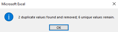
• Step 4: Excel will now delete the duplicate rows and display a dialog box. The dialog box shows a summary of how many duplicate values are found and removed along with the count of unique values. 

• Step 5:  As you can notice, the duplicate records are removed.

Let’s move forward and understand how to remove duplicates in Excel using the Advanced Filter option. 

Understand Filtering for Unique Values or Removing Duplicate Values

With an objective to obtain a list of unique values, you can either filter for unique values or remove duplicate values.

The tasks serve a common purpose. However, there is a critical difference. On filtering for unique values, the duplicate values get temporarily hidden, while the option of removing duplicate values permanently deletes duplicate values.

Also, it is crucial to understand that a comparison of duplicate values relies on what appears in the cell rather than the underlying value contained in the cell.

For instance, if two cells with the same date value are formatted as “4/3/2024” and “Mar 4, 2024”, they are regarded as two unique values.

Therefore, make it a practice to check before removing duplicates. Try to filter or conditionally format unique values to get the expected results.

Why Is Data Validation Important?

The significance of data validation in Excel cannot be overstated. It:

• Ensures that data entered into spreadsheets meets the predefined criteria, reducing the chances of errors.
• Reduces the need for manual checks and corrections of data entries.
• Automates data control, streamlining data entry and processing.
• Maintaining consistency and reliability in datasets is crucial for analysis and decision-making.

Data Validation in Excel

Using data validation in Excel is a powerful way to control the type and values of data entered into your spreadsheets. Properly implemented, data validation can prevent errors, ensure consistent data entry, and make your spreadsheets more professional.

This detailed guide will walk you through how to set up and use data validation in Excel, including tips for advanced use cases.

Step 1: Select the Cells for Data Validation

First, identify the cells where you want to apply data validation. Holding down the Ctrl key while selecting allows you to select a single cell, a range of cells, or multiple non-adjacent cells.

Step 2: Open the Data Validation Dialog Box

To access the data validation settings:

• Click on the cell or cells where you want to apply data validation.
• Go to the Data tab on the Ribbon.
• Click on the Data Validation button in the ‘Data Tools’ group.

This action will open the Data Validation dialog box, which consists of three tabs: Settings, Input Message, and Error Alert.

Step 3: Set Up Validation Criteria

In the Data Validation dialog box, under the Settings tab, you can define your validation criteria:

• Allow: Select the type of data. Options include:
• Whole Number: Only whole numbers are permitted.
• Decimal: Only decimal values are permitted.
• List: Only values from a predefined list are allowed.
• Date: Only date values are permitted.
• Time: Only time values are permitted.
• Text Length: Only text of a certain length is allowed.
• Custom: For more complex criteria, use a formula.
• Data: Specify the condition (e.g., between, not between, equal to, not equal to, etc.).
• Minimum/Maximum: Enter the acceptable range or limits based on your selection above.

For example, to ensure that only values between 10 and 100 are entered in a cell, select “Whole Number,” “between,” and then set the minimum to 10 and the maximum to 100.

Step 4: Configure an Input Message (Optional)

Switch to the Input Message tab to create a message that will appear when the cell is selected:

• Show input message when cell is selected: Check this box to enable the input message.
• Title: Enter a brief title for the input message box.
• Input Message: Type the guidance text that will appear when someone selects the cell. This should instruct them on what type of data to enter.

Step 5: Customize the Error Alert (Optional)

Under the Error Alert tab, you can specify what happens when someone tries to enter invalid data:

• Show error alert after invalid data is entered: Check this to enable error alerts.
• Style: Choose from Stop, Warning, or Information to indicate the severity of the alert.
• Title: Enter a title for the error message box.
• Error Message: Write the message displaying when invalid data is entered. This should explain the error and how to correct it.

Advanced Usage

You can use formulas under the Custom option in the Allow field for more complex validation rules. For example, to validate that the date in a cell is not earlier than today, you could use:

= A1 >= TODAY()

Assuming the validation is being applied in cell A1.

Find value in a range, worksheet or workbook

The following guidelines tell you how to find specific characters, text, numbers or dates in a range of cells, worksheets or entire workbooks.

1. To begin with, select the range of cells to look in. To search across the entire worksheet, click any cell on the active sheet.
   
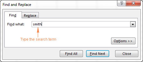
2. Open the Excel Find and Replace dialog by pressing the Ctrl + F shortcut. Alternatively, go to the Home tab > Editing group and click Find & Select > Find.
   

3. In the Find what box, type the characters (text or number) you are looking for and click either Find All or Find Next.

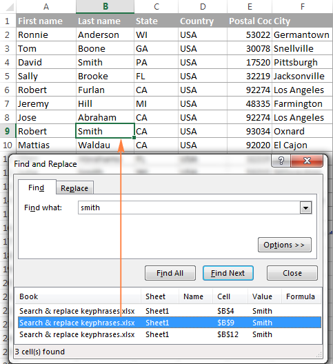
When you click Find Next, Excel selects the first occurrence of the search value on the sheet, the second click selects the second occurrence, and so on.

When you click Find All, Excel opens a list of all the occurrences, and you can click any item in the list to navigate to the corresponding cell.

Excel Find – additional options

To fine-tune your search, click Options in the right-hand corner of the Excel Find & Replace dialog, and then do any of the following:

• To search for the specified value in the current worksheet or entire workbook, select Sheet or Workbook in the Within.
• To search from the active cell from left to right (row-by-row), select By Rows in the Search To search from top to bottom (column-by-column), select By Columns.
• To search among certain data types, select Formulas, Values, or Comments in the Look in.
• For a case-sensitive search, check the Match case check.
• To search for cells that contain only the characters you’ve entered in the Find what field, select the Match entire cell contents.

Find cells with specific format in Excel

To find cells with certain formatting, press the Ctrl + F shortcut to open the Find and Replace dialog, click Options, then click the Format… button in the upper right corner, and define your selections in Excel Find Format dialog box.

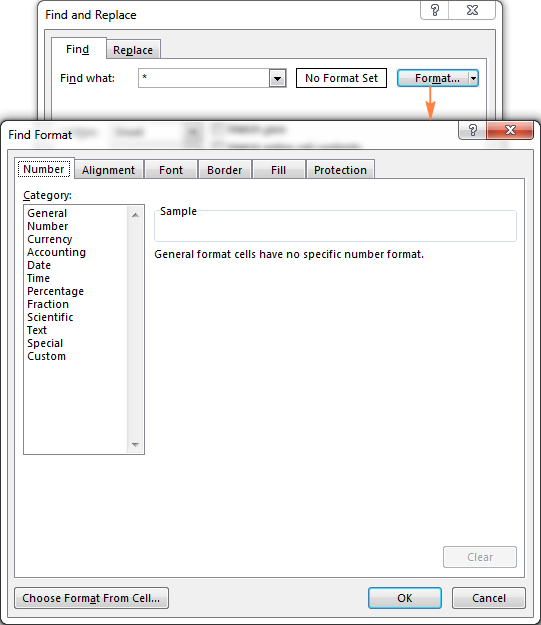
If you want to find cells that match a format of some other cell on your worksheet, delete any criteria in the Find what box, click the arrow next to Format, select Choose Format From Cell, and click the cell with the desired formatting.

Find cells with formulas in Excel

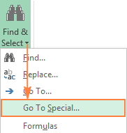
With Excel’s Find and Replace, you can only search in formulas for a given value, as explained in additional options of Excel Find. To find cells that contain formulas, use the Go to Special feature.

1. Select the range of cells where you want to find formulas, or click any cell on the current sheet to search across the entire worksheet.
2. Click the arrow next to Find & Select, and then click Go To Special. Alternatively, you can press F5 to open the Go To dialog and click the Special… button in the lower left corner.
   

3. In the Go To Special dialog box, select Formulas, then check the boxes corresponding to the formula results you want to find, and click OK:

• Numbers – find formulas that return numeric values, including dates.
• Text – search for formulas that return text values.
• Logicals – find formulas that return Boolean values of TRUE and FALSE.
• Errors – find cells with formulas that result in errors such as #N/A, #NAME?, #REF!, #VALUE!, #DIV/0!, #NULL!, and #NUM!.

Conclusion

In wrapping up, Excel’s data handling and formatting features are like a magic wand for anyone working with data. They’re not just about organizing and making data look pretty; they’re about making it easier to understand and use.

Think of Excel as your trusty assistant, helping you sort, filter, and format your data in ways that make sense to you and others. Whether it’s organizing data into tables, highlighting important information with colors and icons, or using formulas to calculate and analyze, Excel has your back.

By taking the time to learn and practice these techniques, you’ll not only save time but also make your data more impactful and meaningful. So, don’t be afraid to dive in, experiment, and see how Excel can transform your data from bland to grand!